Asked in: UBER
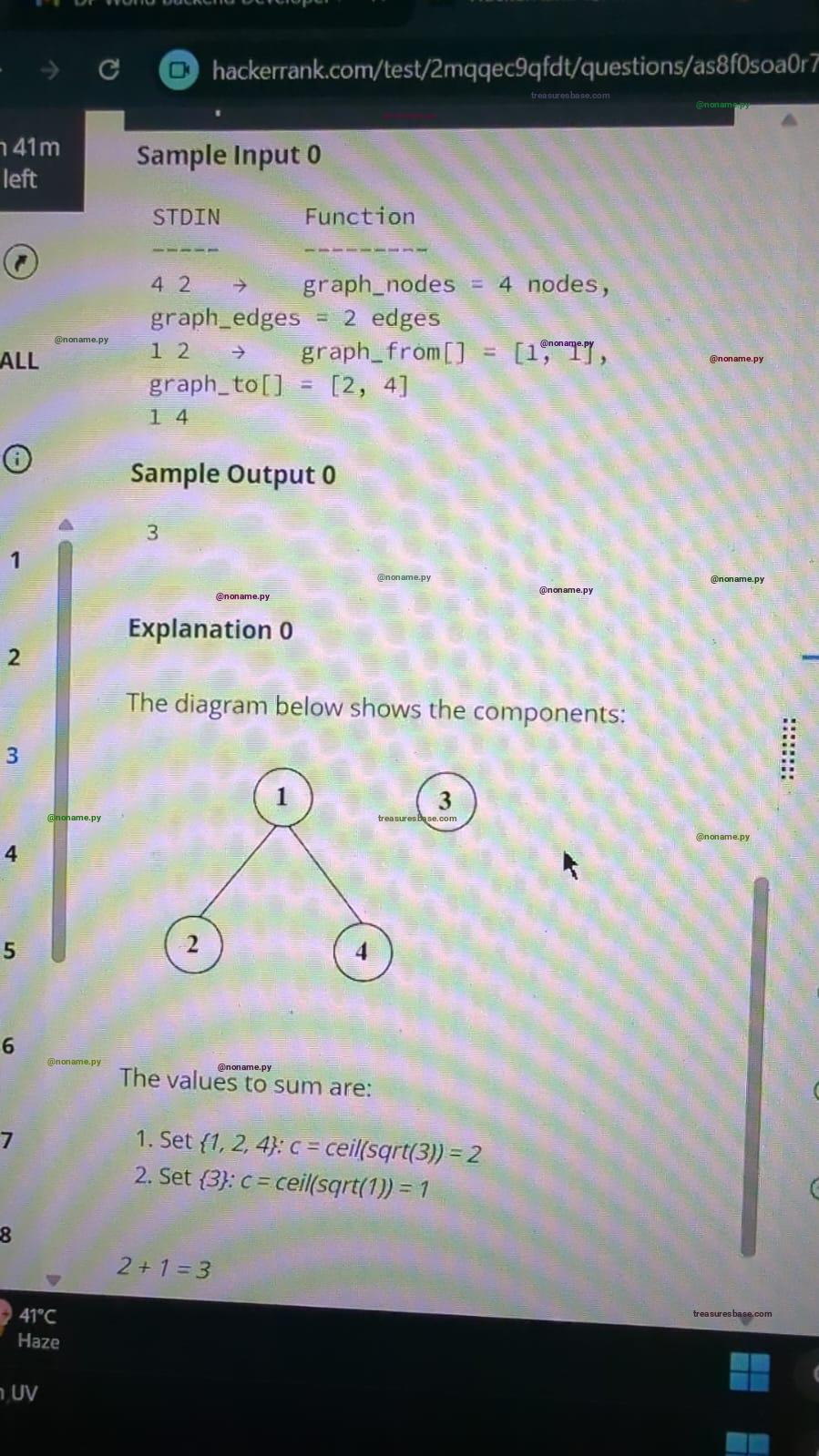
Image of the Question


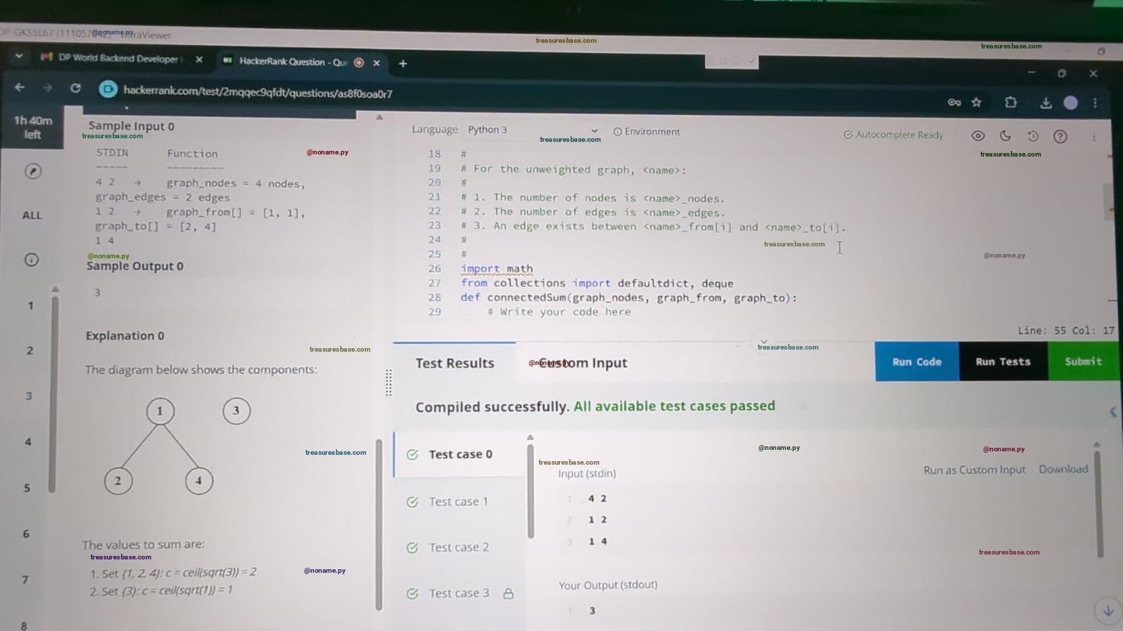
All Testcases Passed ✔
Solution
import math
from collections import defaultdict, deque
def connectedSum(graph_nodes, graph_from, graph_to):
    # Write your code here
// ... rest of solution available after purchaseExplanation
```
To solve this problem, start by understanding the structure and nature of the input: a graph defined by a number of nodes and a list of edges connecting pairs of nodes. The problem requires identifying connected components within this graph, determining their sizes (number of nodes), computing the ceiling of the square root of each size, and finally summing these values across all connected components.
### Step 1: Understand connected components in graphs
A connected component is a subset of nodes where each node is reachable from any other node within the same subset via edges. The entire graph can be divided into one or more such components. Some nodes might be isolated (not connected to any other node), forming components of size one.
### Step 2: Represent the graph efficiently
To find connected components, first represent the graph in a way that facilitates traversal and grouping. Typically, an adjacency list is the most efficient representation for sparse graphs (which is often the case with large nodes and edges). For each node, store a list of neighbors.
### Step 3: Traverse the graph to identify connected components
Once the graph is represented as adjacency lists, use either Depth-First Search (DFS) or Breadth-First Search (BFS) to explore the graph and find connected components:
- Initialize a boolean array or set to keep track of visited nodes.
- For each node in the graph, if it has not been visited, perform DFS/BFS starting from that node.
- Mark all reachable nodes during this traversal as part of the current connected component.
- Count the number of nodes visited in this traversal to find the size of this connected component.
- Store or record this size.
This approach ensures every node is visited exactly once, and each traversal corresponds to exactly one connected component.
### Step 4: Calculate the required value for each component
For each connected component’s size, calculate the ceiling of the square root. The square root gives a measure of the “spread” or “scale” of the component, and the ceiling ensures rounding up to the next integer if the root is not a perfect square. This can be done using standard math functions or binary search to find the smallest integer greater than or equal to the square root.
### Step 5: Sum the values for all components
After calculating the ceil of sqrt for each component, sum these values to get the final answer.
### Step 6: Consider isolated nodes
Nodes that do not appear in any edge list are isolated and hence form connected components of size 1. For these nodes, the ceil of the square root of 1 is simply 1. These should be counted as well.
### Step 7: Optimization considerations
- Since the problem can have up to 10^5 nodes and edges, the solution should be efficient: O(N + E) where N is number of nodes and E is number of edges.
- Use adjacency lists to avoid high memory and time overhead.
- Avoid recursion stack overflow in DFS by using iterative DFS or BFS if necessary.
- Precompute or efficiently calculate square roots for the sizes.
### Step 8: Edge cases and validation
- Check if there are no edges (all isolated nodes).
- Check if the graph is fully connected (one big connected component).
- Verify that nodes mentioned in edges do not exceed the range 1 to graph_nodes.
- Ensure no self loops exist (given constraints).
- Handle multiple disconnected components of varying sizes correctly.
### Summary of the approach:
1. Build adjacency list from edge list.
2. Initialize a visited set or array.
3. For each node from 1 to graph_nodes:
- If not visited, run DFS/BFS to find connected component size.
4. Calculate ceil(sqrt(size)) for each component.
5. Add these values up.
6. Return the sum.
This approach effectively breaks the problem into graph traversal to find connected components and then straightforward mathematical operations to compute the final sum, all within a time complexity suitable for large inputs.
```